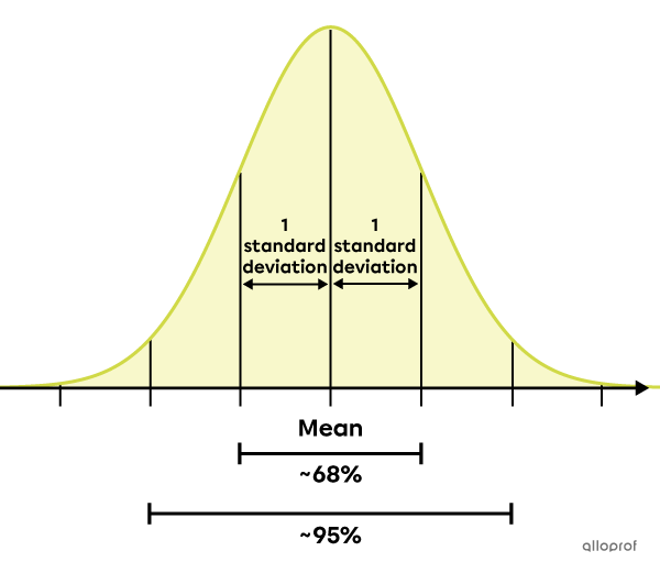
A measure frequently used to study the dispersion of data from the same distribution is the standard deviation.
The standard deviation, usually denoted |s| when studying a sample and |\sigma| when studying a population, is a measure of the dispersion of data around the mean.
In other words, the larger the standard deviation, the further the data are from the mean. Conversely, the smaller the standard deviation, the more concentrated the data are around the mean.
Calculating the standard deviation involves several steps which are summarized by the following formulas:
For a sample
||s= \sqrt{\dfrac{\sum(x_{i}-\overline{x})^{2}}{n-1}}||where
|\overline{x}:| mean of the sample
|n:| size of the sample
For a population
||\sigma = \sqrt{\dfrac{\sum(x_i-\mu)^2}{N}}||where
|\mu:| mean of the population
|N:| size of the population
|\sum| means that you must perform a successive addition of several elements.
|x_i| represents the |i^\text{th}| value of the distribution.
In the standard deviation formula, what is under the square root is called the variance. The calculation of the standard deviation can therefore be summarized by the following equation:
||\text{standard deviation} = \sqrt{\text{variance}}||
In other words, the variance is the mean (average) of the squared deviations from the mean.
Here are the steps to follow to use the above formulas properly:
-
Verify if the distribution is a sample or a population.
-
Determine the size of the distribution.
-
Calculate the mean of the distribution.
-
Calculate the sum of the square of the deviations from the mean.
-
Calculate the standard deviation.
Here are the hourly temperatures (in degrees Celsius) for one day, in ascending order:
|-5,| |-4,| |-4,| |-3,| |-3,| |-2,| |-1,| |0,| |0,| |1,| |2,| |3,| |3,| |4,| |4,| |6,| |7,| |8,| |9,| |10,| |10,| |11,| |11,| |12|
Determine the standard deviation of this distribution.
-
Verify if the distribution is a sample or a population.
This is a sample, since there were times during the day when the temperature was not recorded. Therefore, the formula with |s,| |n,| and |\overline{x}| must be used.
-
Determine the size of the distribution.
Since there are |24| hours in a day, this sample contains |24| data values |(n=24).|
-
Calculate the mean of the distribution.
The arithmetic mean of all the data is calculated.
||\begin{align}\overline{x}&=\dfrac{\left(\begin{alignat}{40}&-5&&-4&&-4&&-\ 3&&-\ 3&&-\ 2&&-\ 1&&+\ 0\\&+0&&+1&&+2&&+\ 3&&+\ 3&&+\ 4&&+\ 4&&+\ 6\\&+7&&+8&&+9&&+10&&+10&&+11&&+11&&+12\ \ \end{alignat}\right)}{24}\\&\approx3.29\end{align}||
-
Calculate the sum of the square of the deviations from the mean.
The deviations from the mean of each data value are calculated and squared.
| Data value |x_i| | Deviation from the mean |\vert x_i-\overline{x}\vert| | Squared deviation from the mean |\left(x_i-\overline{x}\right)^{2}| |
Data value |x_i| | Deviation from the mean |\vert x_i-\overline{x}\vert| | Squared deviation from the mean |\left(x_i-\overline{x}\right)^{2}| |
|---|---|---|---|---|---|
| |-5| | |\vert-5- 3.29\vert=8.29| | |8.29^2\approx68.72| | |3| | |\vert3- 3.29\vert=0.29| | |0.29^2\approx0.08| |
| |-4| | |\vert-4- 3.29\vert=7.29| | |7.29^2\approx53.14| | |4| | |\vert4- 3.29\vert=0.71| | |0.71^2\approx0.50| |
| |-4| | |\vert-4- 3.29\vert=7.29| | |7.29^2\approx53.14| | |4| | |\vert4- 3.29\vert=0.71| | |0.71^2\approx0.50| |
| |-3| | |\vert-3- 3.29\vert=6.29| | |6.29^2\approx39.56| | |6| | |\vert6- 3.29\vert=2.71| | |2.71^2\approx7.34| |
| |-3| | |\vert-3- 3.29\vert=6.29| | |6.29^2\approx39.56| | |7| | |\vert7- 3.29\vert=3.71| | |3.71^2\approx13.76| |
| |-2| | |\vert-2- 3.29\vert=5.29| | |5.29^2\approx27.98| | |8| | |\vert8- 3.29\vert=4.71| | |4.71^2\approx22.18| |
| |-1| | |\vert-1- 3.29\vert=4.29| | |4.29^2\approx18.40| | |9| | |\vert9- 3.29\vert=5.71| | |5.71^2\approx32.60| |
| |0| | |\vert0- 3.29\vert=3.29| | |3.29^2\approx10.82| | |10| | |\vert10- 3.29\vert=6.71| | |6.71^2\approx45.02| |
| |0| | |\vert0- 3.29\vert=3.29| | |3.29^2\approx10.82| | |10| | |\vert10- 3.29\vert=6.71| | |6.71^2\approx45.02| |
| |1| | |\vert1- 3.29\vert=2.29| | |2.29^2\approx5.24| | |11| | |\vert11- 3.29\vert=7.71| | |7.71^2\approx59.44| |
| |2| | |\vert2- 3.29\vert=1.29| | |1.29^2\approx1.66| | |11| | |\vert11- 3.29\vert=7.71| | |7.71^2\approx59.44| |
| |3| | |\vert3- 3.29\vert=0.29| | |0.29^2\approx0.08| | |12| | |\vert12- 3.29\vert=8.71| | |8.71^2\approx75.86| |
The squared deviations from the mean are then added together.
||\begin{alignat}{30}\sum(x_{i}-\overline{x})^{2}&=&&\phantom{\,+\ }68.72&&+53.14&&+53.14&&+39.56&&+39.56&&+27.98\\&&&+18.40&&+10.82&&+10.82&&+5.24&&+1.66&&+0.08\\&&&+0.08&&+0.50&&+0.50&&+7.34&&+13.76&&+22.18\\&&&+32.60&&+45.02&&+45.02&&+59.44&&+59.44&&+75.86\\&=&&\phantom{\,+\ }690.86\end{alignat}||
-
Calculate the standard deviation.
We replace |\boldsymbol{\color{#3b87cd}n}| and |\boldsymbol{\color{#3a9a38}{\sum(x_{i}-\overline{x})^{2}}}| by their respective values in the standard deviation formula for a sample.
||\begin{align}s&=\sqrt{\dfrac{\boldsymbol{\color{#3a9a38}{\sum(x_{i}-\overline{x})^{2}}}}{\boldsymbol{\color{#3b87cd}{n}}-1}}\\&=\sqrt{\dfrac{\boldsymbol{\color{#3a9a38}{690.86}}}{\boldsymbol{\color{#3b87cd}{24}}-1}}\\&=\sqrt{\dfrac{690.86}{23}}\\&\approx\sqrt{30.04}\\&\approx5.48\end{align}||
Answer: The standard deviation of this distribution is about |5.48\ ^\circ \text{C}.|
Note: In this example the variance is |30.04.|
Around 1810, after much research and analysis, the famous mathematician Carl Friedrich Gauss established that, among all possible distributions, many have a data dispersion that tends to follow a specific law. This law is now called Gauss's law, or the normal law. It is therefore referred to as a normal distribution.
He showed that approximately |68\%| of the data of a normal distribution is clustered within |\pm1| standard deviation from the mean and that about |95\%| of the data is located within |\pm2| standard deviations from the mean.
