When the scatter plot of a two variable data distribution demonstrates a linear correlation, the distribution can be modelled by a regression line, often called the “line of best fit.”
The linear regression line is a line that passes through a scatter plot that best represents the 2-variable distribution being studied.
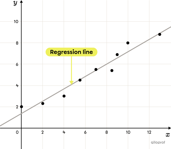
A regression line is used to predict the value of one variable from the value of the other variable through extrapolation or interpolation.
There are several methods for finding the equation of a regression line.
As the name suggests, simply draw a line through the scatter plot so that there are approximately an equal number of points on each side of the line and the slope of the line matches the orientation of the scatter plot as closely as possible.
Later, the rule of the drawn line can be found by using 2 points found on the line itself.
The graphs below show the same scatter plot. In the first one, 3 lines |(y_1,| |y_2,| and |y_3)| have been drawn and they do not constitute proper regression lines, while the lines in the 2nd figure, |(y_4| and |y_5)|, can both be considered valid regression lines.
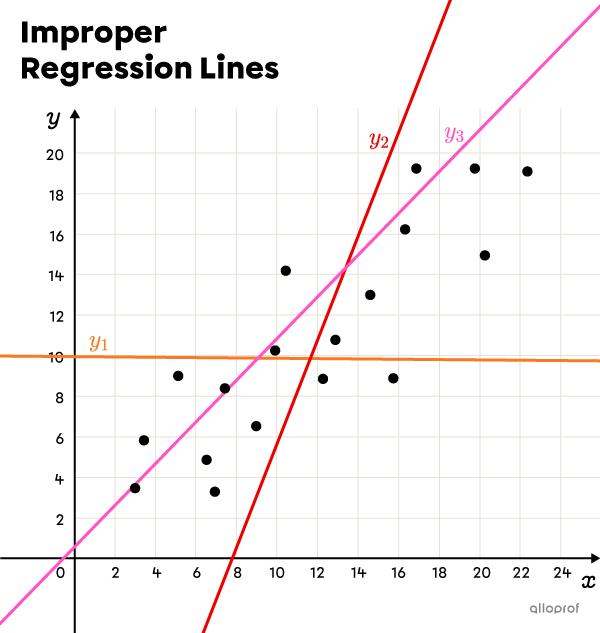
Line |y_1| is not a valid regression line, because it is almost constant, while the scatter plot shows a positive correlation (increasing).
Line |y_2| is not a valid regression line either, because its slope is much steeper than that of the scatter plot.
Line |y_3| has a slope similar to that of the scatter plot, but it does not have an equal number of points on both sides.
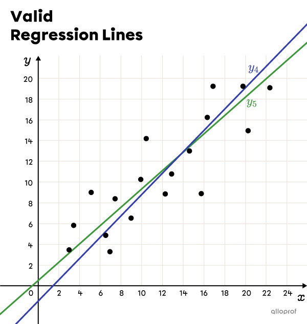
Lines |y_4| and |y_5| are 2 lines that represent the trend of the scatter plot more accurately and have the same number of points on each side. It is possible to use either of these lines to make predictions.
Although the freehand method is acceptable in most situations, it is the least accurate method. As seen in the previous example, 2 lines seem to be appropriate for the same scatter plot, even if they have slightly different slopes. For more accuracy, it is better to use another method such as the Mayer line or the median-median line methods.
The steps to follow to predict data from a scatter plot using the graphing method are as follows:
-
Place the points on a Cartesian plane.
-
Sketch a regression line.
-
Find 2 points that are situated on the regression line.
-
Find the rule of the line using these 2 points.
-
Predict a value using the rule.
Following a survey of |16| Quebec families, total spending on sports and recreation was examined in relation to their household income. The following table of values shows the data collected.
| Household income ($/year) |
|125\ 000| | |65\ 000| | |35\ 000| | |145\ 000| | |130\ 000| | |80\ 000| | |50\ 000| | |40\ 000| |
|---|---|---|---|---|---|---|---|---|
| Spending on sports and recreation ($/year) |
|10\ 000| | |8\ 000| | |1\ 000| | |9\ 000| | |8\ 000| | |6\ 000| | |4\ 000| | |2\ 000| |
| Household income ($/year) |
|90\ 000| | |20\ 000| | |75\ 000| | |105\ 000| | |100\ 000| | |140\ 000| | |150\ 000| | |65\ 000| |
| Spending on sports and recreation ($/year) |
|10\ 000| | |500| | |4\ 000| | |6\ 000| | |8\ 000| | |13\ 000| | |5\ 000| | |5\ 000| |
a) A family has an annual household income of | \$250\ 000.| If this family follows the same trend as the other Quebec families surveyed, how much do they budget for sports and recreation?
b) A family spends an average of | \$7500| a year on sports and recreation. What is their annual household income if they are a typical Quebec family?
-
Place the points on a Cartesian plane.
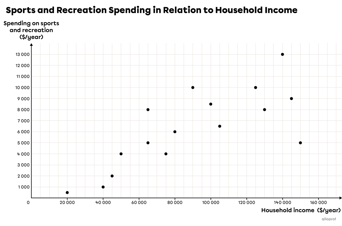
The annual household income is placed on the |x| axis and spending on sports and recreation on the |y| axis.
-
Sketch a regression line.
Since there are |16| points in the scatter plot, we must be sure to place |8| points on either side of the line. We also make sure that the slope of the line best fits the scatter plot.
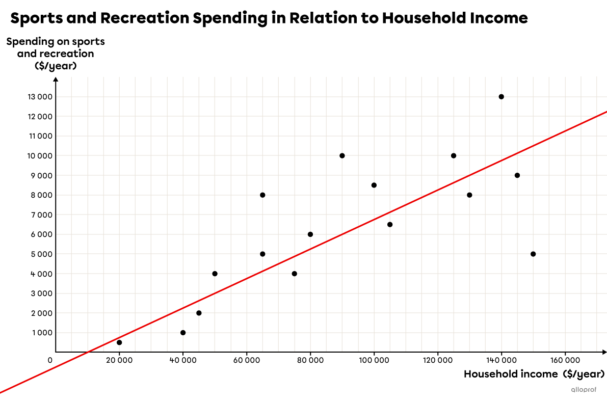
Note: The line could have been drawn a little higher or a little lower. If this is the case, then both the rule and the predictions may slightly vary as a result.
-
Find 2 points situated on the regression line.
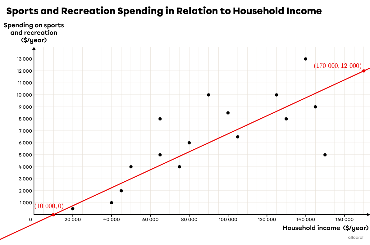
Let’s choose the points |(10\ 000, 0)| and |(170\ 000, 12\ 000).|
-
Find the rule of the line using these 2 points.
Since it is linear, the rule will be of the form |y=ax+b.|
We begin by calculating the slope |(a).| ||\begin{align}a&=\dfrac{y_2-y_1}{x_2-x_1}\\&=\dfrac{12\ 000-0}{170\ 000-10\ 000}\\&=\dfrac{12\ 000}{160\ 000}\\&=\dfrac{3}{40}\\ &=0.075\end{align}|| Next, we replace |a| with |0.075| and the |x| and |y| variables with the coordinates of one of the 2 points, and isolate |b.| ||\begin{align}y&=ax+b\\ y&=0.075x+b\\0&=0.075(10\ 000)+b\\0&=750+b\\-750&=b \end{align}||Therefore, the rule of the regression line that was sketched freehand is |y=0.075x-750.|
-
Predict a value using the rule.
a) A family has an annual household income of |\boldsymbol{\$250\ 000.}| If this family follows the same trend as the other Quebec families surveyed, how much do they budget for sports and recreation?
Since the household income in question | (\$250\ 000)| is outside the range studied (| \$20\ 000| to | \$150\ 000|), this is a prediction by extrapolation.
We replace the |x| variable with |250\ 000| in the regression line rule and complete the calculation. ||\begin{align}y&=0.075x-750\\y&=0.075(250\ 000)-750\\y&=18\ 750-750\\y&=\$ 18\ 000\ \end{align}||
Answer: A household with an annual income of | \$250\ 000| would spend approximately | \$18\ 000| on sports and recreation if it followed the same trend as the other Quebec families surveyed.
b) A family spends an average of |\boldsymbol{\$7\ 500}| a year on sports and recreation. What is their annual household income if they are a typical Quebec family?
This prediction is an interpolation because the annual budget for recreation and sports |( \$7500)| is within the interval studied |(500| to | \$13\ 000).| We can therefore estimate the annual household income of this family using the regression line.
We replace |y| with |7500| and isolate |x.| ||\begin{align} y &= 0.075x-750 \\ 7500 &= 0.075x-750 \\ 7\ 500\boldsymbol{\color{#ec0000}{+750}} &= 0.075x-750\boldsymbol{\color{#ec0000}{+750}} \\ \color{#ec0000}{\dfrac{\color{black}{8250}}{\boldsymbol{0.075}}} &= \color{#ec0000}{\dfrac{\color{black}{0.075x}}{\boldsymbol{0.075}}} \\ 110\ 000\ \$ &= x \end{align}||
Answer: If a household spends on average | \$7500| per year on sports and recreation, we can predict that the household income is about | \$110\ 000.|
In the graph, we can see that the regression line drawn does indeed pass through the point |(110\ 000, 7500).|
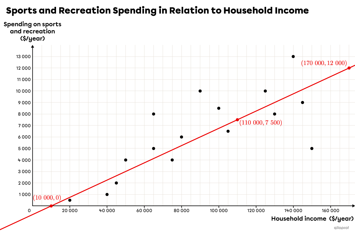
Note: The same problem was solved in the median-median line and Mayer line concept sheets. In each case, comparable results were obtained.
Spreadsheets are software programs used to make tables and graphs. They are programmed to calculate correlation coefficients and to calculate the equation of the line or curve that best fits a given scatter plot.
Spreadsheets are therefore the quickest, most versatile, and most efficient way to find the rule of a regression line and to predict results thereafter.
Following a survey of |16| Quebec families, total spending on sports and recreation was examined in relation to their household income. The following table of values shows the data collected.
| Household income ($/year) |
|125\ 000| | |65\ 000| | |35\ 000| | |145\ 000| | |130\ 000| | |80\ 000| | |50\ 000| | |40\ 000| |
|---|---|---|---|---|---|---|---|---|
| Spending on sports and recreation ($/year) |
|10\ 000| | |8\ 000| | |1\ 000| | |9\ 000| | |8\ 000| | |6\ 000| | |4\ 000| | |2\ 000| |
| Household income ($/year) |
|90\ 000| | |20\ 000| | |75\ 000| | |105\ 000| | |100\ 000| | |140\ 000| | |150\ 000| | |65\ 000| |
| Spending on sports and recreation ($/year) |
|10\ 000| | |500| | |4\ 000| | |6\ 000| | |8\ 000| | |13\ 000| | |5\ 000| | |5\ 000| |
a) A family has an annual household income of | \$250\ 000.| If this family follows the same trend as the other Quebec families surveyed, how much do they budget for sports and recreation?
b) A family spends an average of | \$7500| a year on sports and recreation. What is their annual household income if they are a typical Quebec family?
-
Transcribe the table of values into the spreadsheet.

-
Draw the scatter plot.
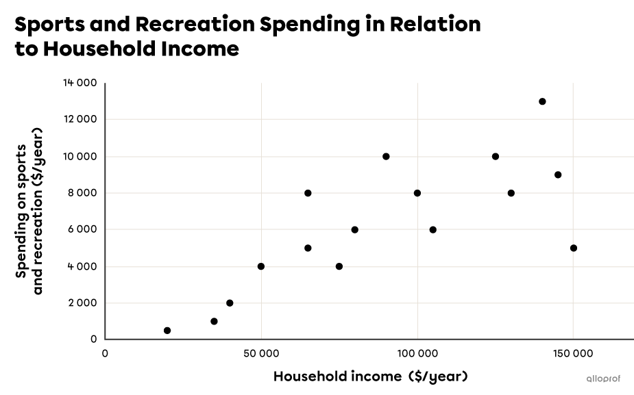
By selecting the cells A1 to Q2, we can ask the software to plot the scatter plot for us in a couple of clicks. The result should look like this:
-
Sketch the regression line.
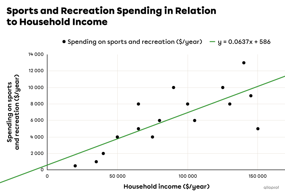
Clicking on the graph gives access to a number of options. One of them is to draw a trend curve. If you choose the linear model, which is often the first model proposed, you get this:
-
Find the rule of the line
We can also decide whether to display the equation of the line or not. In the previous diagram, it appears at the top of the graph.
Therefore, the rule for the regression line found using a spreadsheet is |y=0.063\,7x+586.|
-
Predict a value using the rule.
Generally, software can perform the following calculations automatically. Simply enter an |x| or |y| value and ask the software to predict the value of the other variable using the rule it just calculated.
a) A family has an annual household income of |\boldsymbol{\$250\ 000.}| If this family follows the same trend as the other Quebec families surveyed, how much do they budget for sports and recreation?
We replace the |x| variable with |250\ 000| in the regression line rule and complete the calculation. ||\begin{align}y&=0.0637x+586\\y&=0.0637(250\ 000)+586\\y&=15\ 925+586\\y&=\$16\ 511\ \end{align}||
Answer: A household with an annual income of | \$250\ 000| would spend approximately | \$16\ 511| on sports and recreation if it followed the same trend as the other Quebec families surveyed.
b) A family spends an average of |\boldsymbol{\$7\ 500}| a year on sports and recreation. What is their annual household income if they are a typical Quebec family?
We replace |y| with |7500| in the regression line and isolate |x.|
||\begin{align} y &= 0.0637x+586 \\ 7500 &= 0.0637x+586 \\ 7500\boldsymbol{\color{#ec0000}{-586}} &= 0.0637x+586\boldsymbol{\color{#ec0000}{-586}} \\ \color{#ec0000}{\dfrac{\color{black}{6\ 914}}{\boldsymbol{0.0637}}} &= \color{#ec0000}{\dfrac{\color{black}{0.0637x}}{\boldsymbol{0.0637}}} \\ \$108\ 540\ &\approx x \end{align}||
Answer: If a household spends on average |\$7500| per year on sports and recreation, we can predict that the household income is about |\$108\ 540.|
Note: The same problem was solved in the median-median line and Mayer line concept sheets. In each case, comparable results were obtained.
A prediction made from a scatter plot is never perfectly accurate. This is why, when presenting our predictions, it is best to use the conditional tense. This is also why, when correcting such problems, a margin of error is accepted.
Furthermore, different software programs will not always give exactly the same regression line rule, since they do not necessarily use the same algorithm to calculate it. However, the most common method used by software to calculate a regression line is the least squares method. To find out how this works in practice, please see the following section on this algebraic method.
The method of least squares is an algebraic method that consists of finding the value of the regression line parameters |a| and |b| by trying to minimize the sum of the distances of all the points of the scatter plot from the line in question. To do so, the following formulas must be applied.
Parameter |\boldsymbol{a}| ||a=\dfrac{n\big(\sum x_iy_i\big)-\big(\sum x_i\big)\big(\sum y_i\big)}{n\big(\sum{x_i}^2\big)-\big(\sum{x_i}\big)^2}||
Parameter |\boldsymbol{b}| ||b=\overline{y}-a\overline{x}||
where
|a:| rate of change
|b:| y-intercept
|n:| number of points observed
|\overline{x}:| mean of the x-values
|\overline{y}:| mean of the y-values
|\sum| indicates that we must perform sums of several elements in succession.
|x_i| represents the |i^{\text{th}}| x-value
|y_i| represents the |i^{\text{th}}| y-value
The points on the following Cartesian plane represent the coordinates of 8 houses in a new housing development. The development contractor wants to run a fibre optic network underground as close as possible to each of these houses. Find the equation of the line that represents the optimal position of the underground fibre optic.
| House | |\boldsymbol{x}| Coordinate | |\boldsymbol{y}| Coordinate |
|---|---|---|
| A | |10| | |30| |
| B | |25| | |20| |
| C | |50| | |70| |
| D | |65| | |60| |
| E | |120| | |90| |
| F | |40| | |45| |
| G | |80| | |90| |
| H | |100| | |70| |
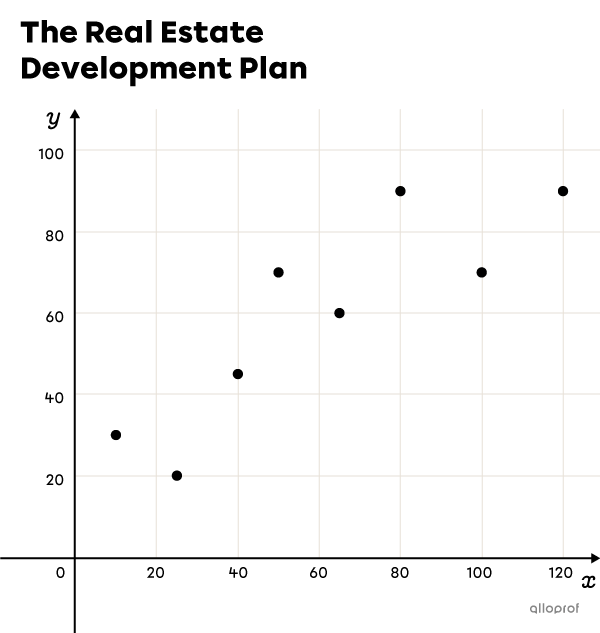
To help us use the formulas of the algebraic method, we start by completing the following table:
| House | |\boldsymbol{x}| Coordinate | |\boldsymbol{y}| Coordinate | |\boldsymbol{xy}| | |\boldsymbol{x^2}| |
|---|---|---|---|---|
| A | |10| | |30| | |300| | |100| |
| B | |25| | |20| | |500| | |625| |
| C | |50| | |70| | |3\ 500| | |2\ 500| |
| D | |65| | |60| | |3\ 900| | |4\ 225| |
| E | |120| | |90| | |10\ 800| | |14\ 400| |
| F | |40| | |45| | |1\ 800| | |1\ 600| |
| G | |80| | |90| | |7\ 200| | |6\ 400| |
| H | |100| | |70| | |7\ 000| | |10\ 000| |
| Sum | |\sum x_i=490| | |\sum y_i=475| | |\sum x_iy_i=35\ 000| | |\sum{x_i}^2=39\ 850| |
| Mean | |\begin{align}\overline{x}&=\dfrac{490}{8}\\&=61.25 \end{align}| | |\begin{align}\overline{y}&=\dfrac{475}{8}\\&=59.375 \end{align}| |
We now apply the formula to calculate the rate of change |(a)| of the regression line. ||\begin{align}a&=\dfrac{n\big(\sum x_iy_i\big)-\big(\sum x_i\big)\big(\sum y_i\big)}{n\big(\sum{x_i}^2\big)-\big(\sum{x_i}\big)^2}\\&=\dfrac{8(35\ 000)-(490)(475)}{8(39\ 850)-(490)^2}\\ &=\dfrac{47\ 250}{78\ 700}\\ &\approx 0.6\end{align}||
We calculate the y-intercept |(b)| using the 2nd formula. ||\begin{align}b&=\overline{y}-a\overline{x}\\&=59.375-0.6(61.25)\\&\approx 22.6\end{align}||
The rule of the regression line is therefore
|y=0.6x+22.6.|
Therefore, by running the main fibre optic cable along this straight line, the contractor minimizes the overall distance from the houses to the cable.

This concept sheet, as well as those on the Mayer and median-median lines, show how to first find the rule of a regression line and then how to use this rule to make predictions.
Making a prediction means finding a new value from the data used to establish a mathematical model. A prediction can be made through interpolation or extrapolation.
-
Interpolation consists of estimating the value of one of the 2 variables under study using the value of the other variable whose value is known and lies within the range covered by the sample data.
-
Extrapolation consists of predicting the value of one of the 2 variables under study from the value of the other variable whose value is known and lies outside the range covered by the sample data.
In general, interpolation is considered more reliable than extrapolation. For example, a given scatter plot may appear to follow a linear pattern, when in fact it follows a quadratic, exponential or other pattern.
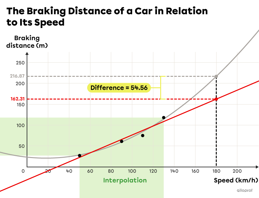
In the graph above, the braking distance of a car is shown as a function of its speed. This phenomenon follows a quadratic pattern. You can see that over the interval covered by the scatter plot, or from |50| to |130\ \text{km/h},| the regression line that models the scatter plot and the actual curve are very close to each other. So, if we use the regression line to interpolate the braking distance of a car travelling between |50| and |130\ \text{km/h},| we get a value that is very close to the actual value.
On the other hand, if the regression line is used to predict the braking distance of a car travelling at |180\ \text{km/h},| by extrapolation, that is, beyond the range studied, the obtained value would be far from the real value.
In other words, just because a scatter plot shows a linear trend does not mean that the same trend continues beyond the scatter plot.
The problem about spending on sports and recreation in relation to household income has been solved using several methods. In the following summary table, we can compare the different results obtained.
|
|
Rule obtained |
Extrapolation |
Interpolation |
|
The Graphing Method (freehand drawing) |
|y=0.075x-750| |
| \$18\ 000| |
| \$110\ 000| |
|
The Least Squares Method (algebraic method) |
|y=0.0637x+586| |
| \$16\ 511| |
| \$108\ 540| |
|
|y=0.07x+6| |
| \$17\ 506| |
| \$107\ 057| |
|
|
|y=0.07x-183| |
| \$17\ 317| |
| \$109\ 757| |
We see that the rules are similar. The rates of change are very close, but it is the initial values that vary the most. The following graph shows the scatter plot and the 4 regression lines obtained using the different methods.
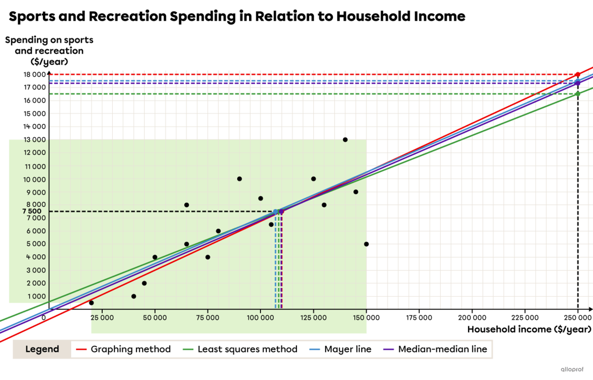
For extrapolation, the estimates range from | \$16\ 511| to | \$18\ 000.| For interpolation, they range from | \$107\ 057| to | \$110\ 000.| If the scatter plot had a stronger correlation, that is, with a correlation coefficient |(r)| closer to |1,| the predictions would have been even closer together.
Finally, since there are no outliers in the data distribution, the Mayer line method is no less reliable than the others.