The Median-Median line method is a procedure for generating a regression line for a given scatter plot by using medians. This line can be used to interpolate or extrapolate values, that is, to make predictions.
The following steps are used to find the rule of the Median-Median line and to make predictions from a 2-variable data set.
-
Order the coordinates according to the independent variable.
-
Separate the distribution into 3 equal groups, if possible.
-
Calculate the median points of each group |(M_1, M_2,| and |M_3).|
-
Calculate the mean point |P,| whose coordinates are the mean of the x-coordinates and the mean of the y-coordinates of the median points.
-
Find the rate of change |(a)| of the line that passes through |M_1| and |M_3.|
-
Find the y-intercept |(b)| of the line that passes through |P| and for which the rate of change is |a.|
-
Predict values using the rule of the line.
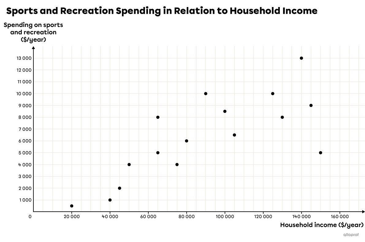
Following a survey of |16| Quebec families, the total spending on sports and recreation was examined in relation to their household income.
The following table of values shows the data collected. The data was then placed on a Cartesian plane to create a scatter plot.
| Household income ($/year) |
|125\ 000| | |65\ 000| | |35\ 000| | |145\ 000| | |130\ 000| | |80\ 000| | |50\ 000| | |40\ 000| |
|---|---|---|---|---|---|---|---|---|
| Spending on sports and recreation ($/year) |
|10\ 000| | |8\ 000| | |1\ 000| | |9\ 000| | |8\ 000| | |6\ 000| | |4\ 000| | |2\ 000| |
| Household income ($/year) |
|90\ 000| | |20\ 000| | |75\ 000| | |105\ 000| | |100\ 000| | |140\ 000| | |150\ 000| | |65\ 000| |
| Spending on sports and recreation ($/year) |
|10\ 000| | |500| | |4\ 000| | |6\ 000| | |8\ 000| | |13\ 000| | |5\ 000| | |5\ 000| |

a) A family has an annual household income of | \$250\ 000.| If this family follows the same trend as the other Quebec families surveyed, how much do they budget for sports and recreation?
b) A family spends an average of | \$7500| a year on sports and recreation. What is their annual household income if they are a typical Quebec family?
-
Order the coordinates according to the independent variable.
| Household income ($/year) |
|20\ 000| | |35\ 000| | |40\ 000| | |50\ 000| | |65\ 000| | |65\ 000| | |75\ 000| | |80\ 000| |
|---|---|---|---|---|---|---|---|---|
| Spending on sports and recreation ($/year) |
|500| | |1\ 000| | |2\ 000| | |4\ 000| | |5\ 000| | |8\ 000| | |4\ 000| | |6\ 000| |
| Household income ($/year) |
|90\ 000| | |100\ 000| | |105\ 000| | |125\ 000| | |130\ 000| | |140\ 000| | |145\ 000| | |150\ 000| |
| Spending on sports and recreation ($/year) |
|10\ 000| | |8\ 000| | |6\ 000| | |10\ 000| | |8\ 000| | |13\ 000| | |9\ 000| | |5\ 000| |
-
Separate the distribution into 3 equal groups, if possible.
Since the number of data sets |(16)| is not evenly divisible by |3,| the groups must be separated so that the 1st and 3rd groups have the same number of data sets. Therefore, the 1st and 3rd groups have |5| pairs of data each and the 2nd has |6.|
| Household income ($/year) |
|20\ 000| | |35\ 000| | |40\ 000| | |50\ 000| | |65\ 000| | |
|---|---|---|---|---|---|---|
| Spending on sports and recreation ($/year) |
|500| | |1\ 000| | |2\ 000| | |4\ 000| | |5\ 000| | |
| Household income ($/year) |
|65\ 000| | |75\ 000| | |80\ 000| | |90\ 000| | |100\ 000| | |105\ 000| |
| Spending on sports and recreation ($/year) |
|8\ 000| | |4\ 000| | |6\ 000| | |10\ 000| | |8\ 000| | |6\ 000| |
| Household income ($/year) |
|125\ 000| | |130\ 000| | |140\ 000| | |145\ 000| | |150\ 000| | |
| Spending on sports and recreation ($/year) |
|10\ 000| | |8\ 000| | |13\ 000| | |9\ 000| | |5\ 000| |
-
Calculate the median points of each group |\boldsymbol{(M_1, M_2}| and |\boldsymbol{M_3)}|.
Find the median of the |x| and |y| coordinates of each group to form 3 points.
Be careful! The median of the |y| coordinates is not necessarily the value that is associated with the median of the |x| coordinates. The median value of the |y| must be carefully chosen.
| Median of the x-values|\boldsymbol{(x)}| | Median of the y-values |\boldsymbol{(y)}| | Mean point | |
|---|---|---|---|
| 1st group | |x_1=40\ 000| | |y_1=2\ 000| | |M_1(40\ 000,2\ 000)| |
| 2nd group | |\begin{align}x_2&=\dfrac{80\ 000+90\ 000}{2}\\&=85\ 000\end{align}| | |\begin{align}y_2&=\dfrac{6\ 000+8\ 000}{2}\\&=7\ 000\end{align}| | |M_2(85\ 000,7\ 000)| |
| 3rd group | |x_3=140\ 000| | |y_3=9\ 000| | |M_3(140\ 000,9\ 000)| |
-
Calculate the mean point |\boldsymbol{P},| whose coordinates are the mean of the x-coordinates and the mean of the y-coordinates of the points |\boldsymbol{M_1, M_2,}| and |\boldsymbol{M_3}|.
||\begin{align}&P\left(\dfrac{x_1+x_2+x_3}{3},\dfrac{y_1+y_2+y_3}{3}\right)\\ &P\left(\dfrac{40\ 000+85\ 000+140\ 000}{3},\dfrac{2000+7000+9000}{3}\right)\\ &P\ \left(88\ 333.\overline{3},6000\right)\end{align}||
-
Find the rate of change |\boldsymbol{(a)}| of the line that passes through |\boldsymbol{M_1}| and |\boldsymbol{M_3}|.
||\begin{align}a&=\dfrac{y_3-y_1}{x_3-x_1}\\&=\dfrac{9000-2000}{140\ 000-40\ 000}\\&=0.07\end{align}||
-
Find the y-intercept |\boldsymbol{(b)}| of the line that passes through |\boldsymbol{P}| and for which the rate of change is |\boldsymbol{a}|.
||\begin{align}y&=ax+b\\ y&=0.07x+b\\ 6000&=0.07(88\ 333.\overline{3})+b\\6000&\approx 6183+b\\-183&\approx b\end{align}||
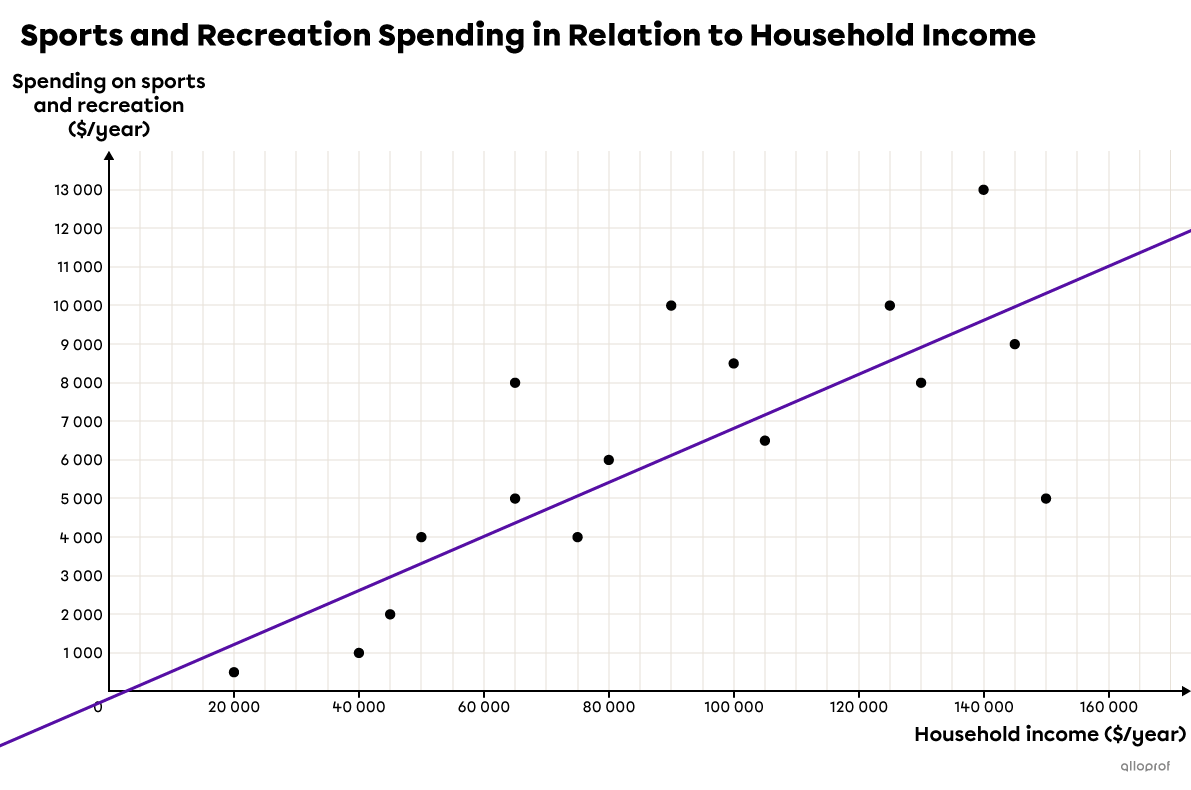
So, the rule of the Median-Median line is |y=0.07x-183,| where |x| is the household income and |y| is the spending on sports and recreation, both in |\$| per year. We can graph this line.

-
Predict values using the rule of the line.
a) A family has an annual household income of | \$250\ 000.| If this family follows the same trend as the other Quebec families surveyed, how much do they budget for sports and recreation?
We can estimate this family's spending on sports and recreation using the regression line. Since the family income in question | \$250\ 000| is outside the range studied, (| \$20\ 000| to | \$150\ 000|), this is an extrapolation.
We replace the |x| variable with |250\ 000| in the regression line rule and complete the calculation. ||\begin{align}y&=0.07x-183\\y&=0.07(250\ 000)-183\\y&=17\ 500-183\\y&=\$17\ 317\ \end{align}||
Answer: A household with an annual income of | \$250\ 000| would spend approximately | \$17\ 317| on sports and recreation if it followed the same trend as the other Quebec families surveyed.
b) A family spends an average of |\$7500| a year on sports and recreation. What is their annual household income if they are a typical Quebec family?
We can estimate the annual household income of this family using the regression line. This is an interpolation because the annual budget for recreation and sports |( \$7500)| is within the interval studied |(500| to |\$13\ 000).|
We replace |y| with |7500| and isolate |x.| ||\begin{align} y &= 0.07x-183 \\ 7500 &= 007x-183 \\ 7500\boldsymbol{\color{#ec0000}{+183}} &= 0.07x-183\boldsymbol{\color{#ec0000}{+183}} \\ \dfrac{7683}{\boldsymbol{\color{#ec0000}{0.07}}} &= \dfrac{0.07x}{\boldsymbol{\color{#ec0000}{0.07}}} \\ \$109\ 757\ &\approx x \end{align}||
Answer: If a household spends on average |\$7500| per year on sports and recreation, we can predict that the household income is about |\$109\ 757.|
Note: The same problem was solved in the regression line and Mayer line concept sheets. In each case, comparable results were obtained.
When the points need to be ordered
-
Points are ordered according to their x-coordinates. You should not order the x- and y-coordinates separately.
-
If 2 points have the same x-coordinate, but different y-coordinates, the one with the smaller y-coordinate is placed first.
Example:
Here is a table of values.
| |x| | |13| | |12| | |13| | |13| | |10| | |12| |
|---|---|---|---|---|---|---|
| |y| | |35| | |24| | |35| | |28| | |25| | |29| |
We get the following table.
| |x| | |10| | |12| | |12| | |13| | |13| | |13| |
|---|---|---|---|---|---|---|
| |y| | |25| | |24| | |29| | |28| | |35| | |35| |
We do not get this one.
| |x| | |10| | |12| | |12| | |13| | |13| | |13| |
|---|---|---|---|---|---|---|
| |y| | |24| | |25| | |28| | |29| | |35| | |35| |
When the points need to be separated into 2 groups
-
If the number of points can be divided evenly by |3,| the groups are equal.
For example, 18 = 6 + 6 + 6 -
If the number of points cannot be divided evenly by |3,| make sure that the 1st and 3rd groups are the same size, and that the size of all |3| groups are as equal as possible. Here are 2 examples:
-
|29 = 10 + 9 + 10| and not |9 + 11 + 9|
-
|25 = 8 + 9 + 8| and not |9 + 7 + 9|
-
When calculating the median points
-
Since the points are already ordered according to the |x| values, we just need to select the median of |x| in each group.
-
For the |y| values, it is not necessary to use the value that forms a pair with the chosen |x| value. The median of |y| in each group must be selected.
Example:
| 1st group | 2nd group | 3rd group | ||||||||
|---|---|---|---|---|---|---|---|---|---|---|
| |x| | |1| | |\boldsymbol{2}| | |4| | |4| | |\boldsymbol{5}| | |\boldsymbol{6}| | |7| | |7| | |\boldsymbol{8}| | |10| |
| |y| | |5| | |8| | |\boldsymbol{7}| | |9| | |\boldsymbol{10}| | |\boldsymbol{10}| | |13| | |\boldsymbol{16}| | |14| | |20| |
-
In the 1st group, there is an odd number of points. The median x-value is |2.| Since the y-values of this group are |5,| |7| and |8,| the median y-value of this group is |\boldsymbol{7}| and not |8.| Therefore, point |M_1| has coordinates |(2,7)| even though point |(2,7)| is not part of the scatter plot.
-
In the 2nd group, there is an even number of data.||\begin{align} x_2 &= \dfrac{5+6}{2}=5.5 \\ y_2 &=\dfrac{10+10}{2}=10 \end{align}|| So, the point |M_2| is |(5.5, 10).|
-
In the 3rd group, |x_3=8| and |y_3=\boldsymbol{16}| and not |14.| So, point |M_3| is |(8, 16).|
Une erreur s’est glissée dans cette vidéo.
À 7 min 30 s, on devrait lire : les points |M1 (45,54)| et |M3 (92,84).| Le calcul est exact, mais il y a une erreur dans la 1re phrase.
The Median-Median line method generally takes a little longer to complete than the Mayer line method, but that does not mean that it is not a good method. Here is an example where the two approaches are presented in parallel so that they can be compared.
During a hockey season, the points scored by all players are counted. A player's points include both assists and goals. In hockey, up to 2 assists are counted for each goal scored, meaning the last 2 passes made just before the goal.
Here are the numbers of assists and points for 10 regular Boston Bruins forwards during the 2022-2023 NHL season.
| Player | Number of assists | Number of points |
|---|---|---|
| D. Pastrnak | ||49|| | ||109|| |
| B. Marchand | ||46|| | ||66|| |
| P. Zacha | ||37|| | ||58|| |
| P. Bergeron | ||30|| | ||57|| |
| D. Krejci | ||40|| | ||56|| |
| J. DeBrusk | ||23|| | ||48|| |
| C. Coyle | ||29|| | ||44|| |
| T. Hall | ||20|| | ||36|| |
| T. Frederic | ||14|| | ||30|| |
| N. Foligno | ||16|| | ||28|| |
Based on this team's data, a player who made 60 assists should have finished the season with how many points?
-
Order the coordinates according to the independent variable.
| Number of assists | |14| | |16| | |20| | |23| | |29| | |30| | |37| | |40| | |46| | |49| |
|---|---|---|---|---|---|---|---|---|---|---|
| Number of points | |30| | |28| | |36| | |48| | |44| | |57| | |58| | |56| | |66| | |109| |
The Median-Median line
-
Separate the distribution into 3 equal groups, if possible.
The 1st and 3rd groups have |3| data pairs each and the 2nd has |4.|
-
Calculate the median points of each group |\boldsymbol{(M_1, M_2}| and |\boldsymbol{M_3)}|.
| Median of the x-values|\boldsymbol{(x)}| | Median of the y-values |\boldsymbol{(y)}| | Mean point | |
| 1st group | |x_1=16| | |y_1=30| | |M_1(16,30)| |
| 2nd group | |\begin{align}x_2&=\dfrac{29+30}{2}\\&=29.5\end{align}| | |\begin{align}y_2&=\dfrac{48+57}{2}\\&=52.5\end{align}| | |M_2(29.5,52.5)| |
| 3rd group | |x_3=46| | |y_3=66| | |M_3(46,66)| |
-
Calculate the mean point |\boldsymbol{P},| whose coordinates are the mean of the x-coordinates and the mean of the y-coordinates of the points |\boldsymbol{M_1, M_2}| and |\boldsymbol{M_3}|
||P\left(\dfrac{16+29.5+46}{3},\dfrac{30+52.5+66}{3}\right)=(30.5,49.5)||
-
Find the rate of change |\boldsymbol{(a)}| of the line that passes through |\boldsymbol{M_1}| and |\boldsymbol{M_3}|
||\begin{align}a&=\dfrac{y_3-y_1}{x_3-x_1}\\&=\dfrac{66-30}{46-16}\\&=1.2\end{align}||
-
Find the y-intercept |\boldsymbol{(b)}| of the line that passes through |\boldsymbol{P}| and for which the rate of change is |\boldsymbol{a}|
||\begin{align} y &= ax+b \\ y &= 1.2x+b \\ 49.5 &= 1.2(30.5)+b \\ 49.5 &= 36.6+b \\ 12.9 &= b \end{align}||So, the rule of the median-median line is |\color{#560fa5}{y=1.2x+12.9},| where |x| is the number of assists and |y,| the number of points.
-
Predict values using the rule of the line.
The number of points is extrapolated using the median-median line by replacing the |x| variable with |60.|
||\begin{align} y &= 1.2x+12.9 \\&= 1.2(60)+12.9 \\ &= 72+12.9 \\ &= 84.9\\ &\approx 85\ \text{points} \end{align}||
The Mayer line
-
Separate the distribution into 2 equal groups, if possible.
The 1st group is formed by the |5| pairs with a number of assists of |29| or less. The other |5| pairs form the 2nd group.
-
Calculate the mean points of each group |\boldsymbol{(P_1}| and |\boldsymbol{P_2)}|.
| Mean of the x-values |\boldsymbol{(\overline{x})}| | Mean of the y-values |\boldsymbol{(\overline{y})}| | Mean point | |
| 1st group | |\begin{align}\overline{x}_1 &= \dfrac{14+16+20+23+29}{5} \\ &=20.4\end{align}| | |\begin{align}\overline{y}_1 &= \dfrac{30+28+36+48+44}{5} \\ &=37.2\end{align}| | |P_1(20.4, 37.2)| |
| 2nd group | |\begin{align}\overline{x}_2 &= \dfrac{30+37+40+46+49}{5} \\ &=40.4\end{align}| | |\begin{align}\overline{y}_2 &= \dfrac{57+58+56+66+109}{5} \\ &=69.2\end{align}| | |P_2(40.4,69.2)| |
-
Find the rule of the regression line that passes through the points |\boldsymbol{P_1}| and |\boldsymbol{P_2}.|
Since this is a straight line, the rule is of the form |y=ax+b.| We start by calculating the slope |(a).| ||\begin{align}a&=\dfrac{\overline{y}_2-\overline{y}_1}{\overline{x}_2-\overline{x}_1}\\&=\dfrac{69.2-37.2}{40.4-20.4}\\&= 1.6\end{align}|| Next, we replace |a| by |1.6| and the |x| and |y| variables by the coordinates of one of the 2 points. Then, we isolate |b.| ||\begin{align} y &= ax+b \\ y &= 1.6x+b \\ 37.2 &= 1.6(20.4)+b \\ 37.2 &= 32.64+b \\ 4.56 &= b \end{align}|| So, the rule for the regression line found using the Mayer line method is |\color{#3b87cd}{y=1.6x+4.56},| where |x| is the number of assists and |y,| the number of points.
-
Predict values using the rule of the line.
This is an extrapolation, since the number of assists |(60)| is outside the interval studied |(14| to |49).| The number of points can now be estimated using the Mayer line by replacing |x| with |60.| ||\begin{align} y &= 1.6x+4.56 \\&= 1.6(60)+4.56 \\ &= 96+4.56\\&= 100.56\\ &\approx 101\ \text{points} \end{align}||
Answer: A player who makes |60| assists in a season should get about |85| points according to the median-median line or |101| points according to the Mayer line.
The Median-Median method is based on medians, whereas the Mayer method is based on means. The mean, unlike the median, is a measure of central tendency that is heavily influenced by distant data, also known as outliers. As such, outliers do not affect the mean-median line. It is therefore the preferred method when there are outliers in a distribution.
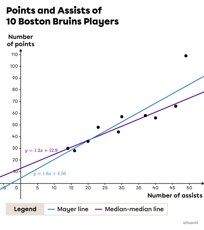
If we go back to the previous example and graph the scatter plot and the 2 lines on the same graph, we can indeed see that the median-median line is less influenced by the outlier than the Mayer line.

First of all, we notice that the slope of the two lines is quite different. The rate of change for the median-median line is |1.2,| whereas the slope of the Mayer line is |1.6.|
We also notice that the point |(49,109),| which represents David Pastrnak's data, is far from the others. This player accumulated far more total points in relation to his number of assists than the rest of his team |\left(\dfrac{109}{49} \approx 2.22\right).|
Pastrnak's data had an impact on the Mayer method, since it was included in the calculation of the mean points. This had the effect of increasing the value of the slope of the Mayer line compared to the other method. The point |(49,109),| even if it is high, does not influence the median points. This is why the median-median line is less steep and fits the data set better, as seen on the graph. On the contrary, the Mayer line is more inclined towards the point |(49,109)| and therefore less fitted to the rest of the scatter plot.
Conclusion: Predictions made using the median-median line are considered to be more representative of all players. So, a player who makes |60| assists in a season should earn about |85| points and not |101.|