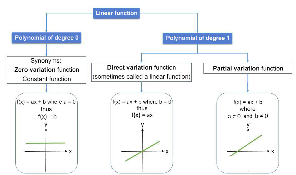
A linear function is a function with a constant rate of change. It’s written in the form |f(x) = ax + b,| where |a| and |b| are real numbers |(\mathbb{R}).|
Graphically, a linear function is represented by a straight line.
Graphs of the lines can vary according to their rate of change (parameter |a| ) and their |y|-intercept (parameter |b|). Therefore, the lines are classified in various categories.

A zero-degree polynomial function (zero variation) is a function that does not vary. It will always be equal to a number. Variations of the independent variable |(x)| do not lead to variations of the dependent variable |(y).|
A zero-degree polynomial function of equation is written in the following form. ||f(x) = b|| where |b| is a constant
The rule comes from the general rule for linear functions: |f(x) = ax + b.|
-
However, since the rate of change is zero, the parameter |a| is equal to |0.| Therefore, the rule becomes |f(x) = b|. Since the dependent variable |(y)| is always constant, the table of values of a zero variation function is marked by a constant value |y|.
-
The graphical representation of this function is a line parallel to the |x|-axis intersecting the |y|-axis at |(0,b)|.
Consider the following zero variation situation:
Regardless of the variable’s variation, |x|, the value of |y| is always the same, |4|.
The function can be represented using the rule |y=4|, a table of values (below left), or by a graph (below right).
|
|x| |
|y| |
|---|---|
|
|5| |
|4| |
|
|3| |
|4| |
|
|0| |
|4| |
|
|-2| |
|4| |
A direct variation function (first-degree polynomial) is a function which reflects a situation of proportionality. Therefore, constant variations of the independent variable |(x)| lead to constant and non-zero variations of the dependent variable |(y)|.
A first-degree polynomial function of of direct variation’s function is written as follows: ||f(x) = ax|| where |a\neq 0|
The rule comes from the general rule for linear functions: |f(x) = ax + b| . However, since the direct variation situation is proportional, the |y|-intercept |(b)| is zero because the line passes through |(0,0)|.
-
Therefore, the parameter |b| is equal to |0|. So, the rule becomes |f(x) = ax|. The direct variation function passes through the point |(0,0)|.
-
A direct variation function’s table of values is characterized by the presence of the coordinate |(0,0)|.
-
The graphical representation of the function is an oblique line that intersects the |y|-axis at |(0,0)|.
Consider the following direct variation situation:
A bathtub, empty at first, fills at the rate of 5 litres of water per minute. We want to represent the number of litres of water in the bathtub as a function of time in minutes.
The function can be represented using the rule |f(x)=5x| , where |x| is the time in minutes and |f(x)| is the number of litres.
It can also be represented by a table of values (below left) or by a graph (below right).
|
|x| |
|y| |
|---|---|
|
|0| |
|0| |
|
|2| |
|10| |
|
|4| |
|20| |
|
|6| |
|30| |
A partial variation function (first-degree polynomial) is a function where constant variations of the independent variable |(x)| lead to constant and non-zero variations of the dependent variable |(y)|. However, unlike the direct variation function, it does not reflect a situation of proportionality since it does not pass through |(0,0)| .
A first-degree polynomial function of a partial variation equation is written as follows:||f(x) = ax + b||where |a\neq 0| and |b\neq 0|
The rule corresponds to the general rule for linear functions: |f(x) = ax + b.|
The equation of a line can also be written in other forms. For more information, see the following link: Forms of the Equation of a Line.
-
The partial variation function does not pass through point |(0,0).| Instead, it intersects the |y|-axis at point |(0,b)| .
-
A partial variation function’s table of values has an initial non-zero value.
-
The graphical representation of the function is an oblique line that does not pass through the origin of the Cartesian plane.
Consider the following partial variation situation.
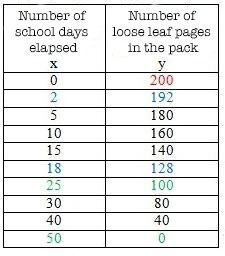
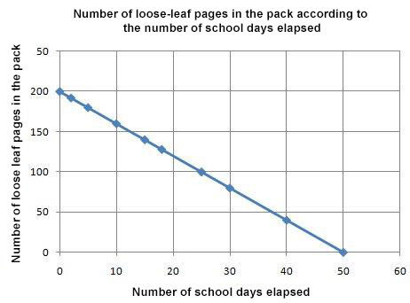
Mark buys a pack of 200 loose-leaf sheets at the start of the school year. He uses an average of 4 sheets each school day. We are interested in the number of sheets left in his pack, depending on the number of school days elapsed.
The partial variation can be represented by the rule |f(x) = -4x + 200.|
It can also be represented by a table of values (below left) or by a graph (below right).

| |\boldsymbol{x:}| Number of school days elapsed | |\boldsymbol{f(x):}| Number of loose leaf pages in the pack |
|---|---|
| 0 | 200 |
| 2 | 192 |
| 5 | 180 |
| 10 | 160 |
| 15 | 140 |
| 18 | 128 |
| 25 | 100 |
| 30 | 80 |
| 40 | 40 |
| 50 | 0 |
