In a Cartesian plane, a linear function is represented by a line. It is generally drawn using a table of values or using parameters |a| and |b.|
When sketching a linear function, it is necessary to determine at least two points which satisfy it. However, it may be beneficial to find additional points for a more accurate graph.
Follow these steps to graph a linear function from a table of values.
-
Create the table of values.
-
Plot the points in a Cartesian plane.
-
Draw the line.
To build a table of values, place the |x| values in ascending order. It is not necessary to have regular jumps between each value.
Sketch the linear function with the rule |y=2x-4.|
-
Create the table of values
We assign random values to |x| and then determine the corresponding value of |y.|
We use |x=1.| ||\begin{align}y&=2\color{#3B87CD}x-4\\y&=2(\color{#3B87CD}{1})-4\\y&=2-4\\y&=-2 \end{align}|| When |x=1,| |y=-2.| Therefore, the first point is |(1,-2).|
We continue by choosing a different |x| value. We use |x=0.|||\begin{align}y&=2\color{#3B87CD}x-4\\y&=2(\color{#3B87CD}{0})-4\\y&=0 -4\\y&=-4\end{align}|| Therefore, the second point is |(0,-4).|
| |x| | |y| |
|---|---|
| |-1| | |-6| |
| |0| | |-4| |
| |1| | |-2| |
| |3| | |2| |
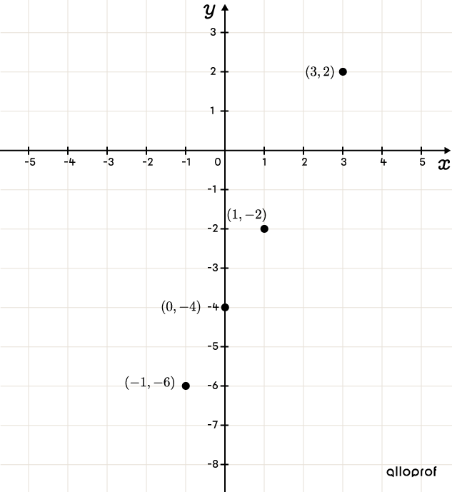
We continue building the table of values in the same way to determine more points. We get the points |(3,2)| and |(-1,-6).|
-
Plot the points in a Cartesian plane
We draw the |x|-axis and the |y|-axis. The appropriate scale is determined by the points found in the previous step. Here, a scale of |1| unit works well.
-
Draw the line
Using a ruler, we connect the points to draw the line that represents the linear function.
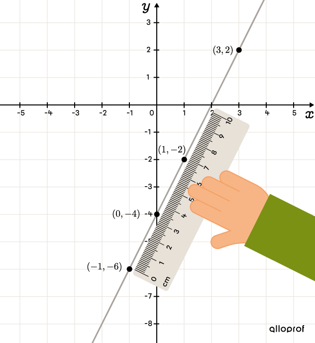
To fully use the Cartesian plane, we generally choose both negative and positive |x| values. Additionally, choosing |x=0| is a good strategy given that the determined value corresponds to the |y|-intercept (i.e., where the line intersects |y|-axis).
Finally, since a linear function extends to infinity, we must extend the line before and after the chosen points.
The graph of a linear function can be drawn using its parameters. In fact, parameter |a| is the rate of change (also called the slope) and parameter |b| corresponds to the |y|-intercept (also called the initial value). These two pieces of information are sufficient to graph the function. Proceed as follows.
-
Place the |y|-intercept |(b).|
-
Place the next point(s) using the rate of change |(a).| To do this, use the formula for calculating the slope. ||a=\dfrac{\Delta y}{\Delta x}=\dfrac{\text{Change in }y}{\text{Change in }x}||
-
Draw the line.
When the rate of change is positive, |y| moves up in the Cartesian plane and |x| moves to the right. ||\color{#EC0000}+a=\dfrac{\color{#EC0000}+\Delta y}{\color{#EC0000}+\Delta x}||
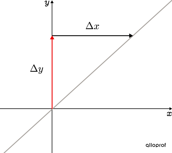
When the rate of change is negative, |y| moves down in the Cartesian plane and |x| moves to the right. ||\color{#EC0000}-a=\dfrac{\color{#EC0000}-\Delta y}{\color{#EC0000}+\Delta x}||
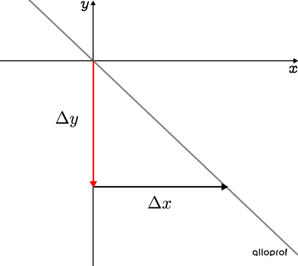
Sketch the linear function with the rule |y=-\dfrac{3}{2}x+1.|
-
Place the |y|-intercept |(b)|
The |y|-intercept corresponds to the constant term in the rule. ||\begin{align}y&=ax+\color{#3A9A38}b\\y&=-\dfrac{3}{2}x+\color{#3A9A38}1\end{align}||||\color{#3A9A38}b=\color{#3A9A38}1||
The |y|-intercept is at point |(0,1).|
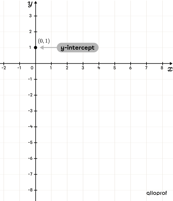
-
Place the next points according to the rate of change
The rate of change corresponds to the coefficient of variable |x| in the rule. ||\begin{align}y&=\color{#3B87CD}ax+b\\y&=\color{#3B87CD}{-\dfrac{3}{2}}x+1\\\\\color{#3B87CD}{a}&=\color{#3B87CD}{-\dfrac{3}{2}}\end{align}||
We use the slope formula. ||\begin{align}a=\dfrac{\color{#FA7921}{-3}}{\color{#FF55C3}2}=\dfrac{\color{#FA7921}{\text{Change in }y}}{\color{#FF55C3}{\text{Change in }x}}\end{align}||From the |y|-intercept, we must descend |\color{#FA7921}3| units, and then move |\color{#FF55C3}2| units to the right. We get the point |(2,-2).|
By repeating the same process from the point |(2,-2),| we get points |(4,-5)| and |(6,-8).|
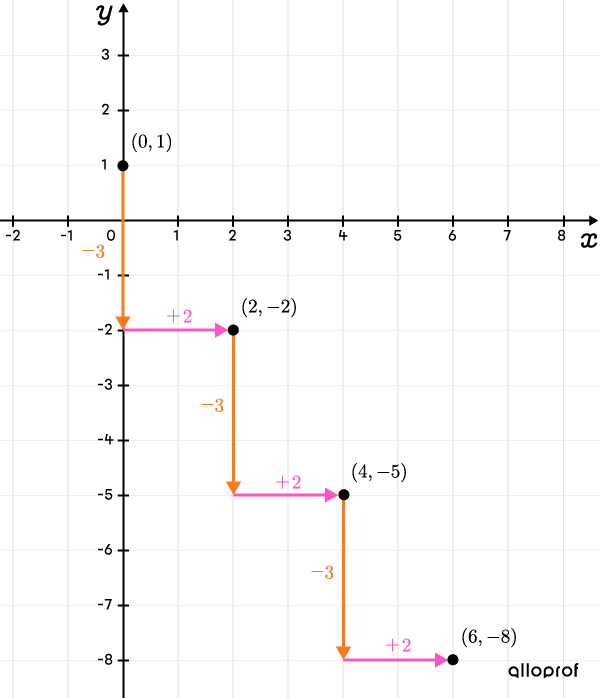
-
Draw the line
Using a ruler, we connect the points to draw the line that represents the linear function.
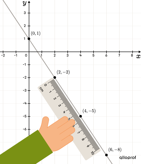
When the rate of change is written in decimal notation, it helps to change it to fractional notation. Moreover, if |a| is negative, the numerator of the fraction is negative.
For example:
If |a=2{.}5,| write |a=\dfrac{5}{2}.|
If |a=4,| write |a=\dfrac{4}{1}.|
If |a=\color{#EC0000}{-}\dfrac{4}{3},| write |a=\dfrac{\color{#EC0000}{-}4}{3}.|
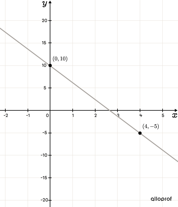
Sketch the linear function with the rule |y=-3{.}75x+10.|
-
Place the |y|-intercept |(b)|
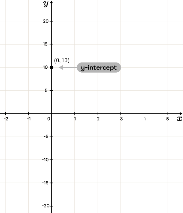
||\begin{align}y&=ax+\color{#3A9A38}b\\y&=-3{.}75x+\color{#3A9A38}{10}\end{align}||||\color{#3A9A38}b=\color{#3A9A38}{10}||The |y|-intercept is at point |(0,10).|
-
Place the next points according to the rate of change||\begin{align}y&=\color{#3B87CD}ax+b\\y&=\color{#3B87CD}{3{.}75}x+10\end{align}|| We convert decimal notation to fractional notation. ||\color{#3B87CD}{a}=\color{#3B87CD}{-3{.}75}=\color{#3B87CD}{\dfrac{-15}{4}}||
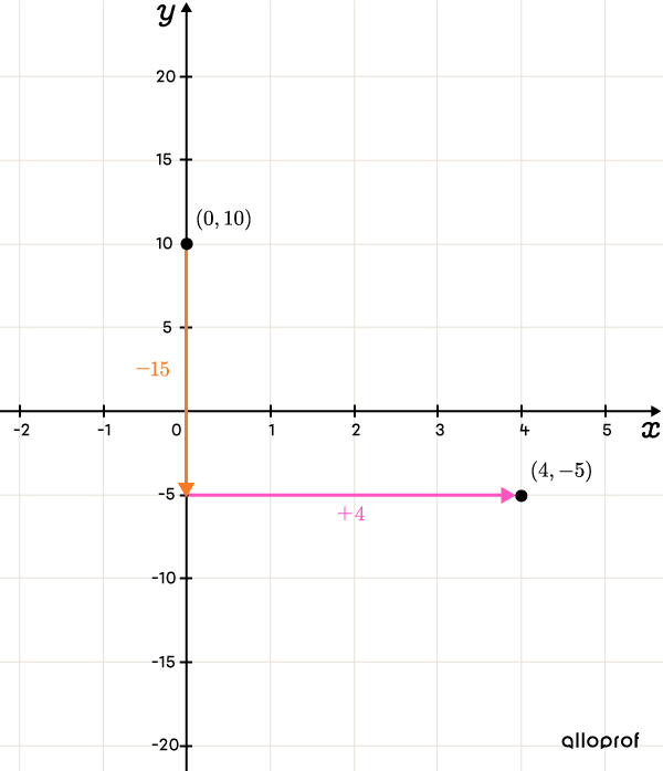
We use the slope formula. ||\begin{align}a=\dfrac{\color{#FA7921}{-15}}{\color{#FF55C3}4}=\dfrac{\color{#FA7921}{\text{Change in }y}}{\color{#FF55C3}{\text{Change in }x}}\end{align}|| From the |y|-intercept, we must descend |\color{#FA7921}{15}| units, and then move |\color{#FF55C3}{4}| units to the right.
When the rate of change indicates a large variation, it is necessary to change the scale. Here, we can make leaps of |5| units in |y| and |1| unit in |x.| In this way, we descend the equivalent of |3| squares only. We get the point |(4,-5).|
-
Connect the points
Using a ruler, we connect the points to draw the line that represents the linear function.
